MauroCerbai

Come ho costruito un database SQLite parsificando i dati dei pokemon disponibili sulle guide online

function getPkList(tbl, array){

    $(tbl).find('tr').each(function (i) { //loop on each tr in table

        // SKIP HEADER

        if(i===0) return;

        //CREATE POKEMON OBJECT

        var poke = {};

        var $tds = $(this).find('td'); //get all td tags

        poke.strid = $tds.eq(1).text(); //access first td and get text content

        poke.strid = poke.strid.replace('#','');

        poke.id = parseInt(poke.strid, 10);

        poke.imageUrl = $tds.eq(2).find('img')[0].getAttribute('src'); //access second td and get src attribute of the img tag

        poke.name = $tds.eq(3).find('a')[0].text;

        poke.type1 = $tds.eq(4)[0].innerText;

        if($tds.eq(5)[0])

            poke.type2 = $tds.eq(5)[0].innerText;

        array.push(poke); //save object to the array

    });

}

Struttura del database

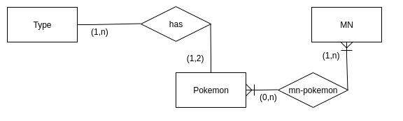
Import dei dati in database

• crea le tabelle del database

db.prepare(`CREATE TABLE IF NOT EXISTS \`types\` (

  \`id\` INT NOT NULL, \`name\` VARCHAR(100) NOT NULL,

   PRIMARY KEY (\`id\`));`).run();

• leggo il json e ciclo su ogni valore

let pokelist = JSON.parse(fs.readFileSync('./data/pokedex_list.json', 'utf8'));

for (let index in pokelist) {

• verifico se il tipo è già presente altrimenti l'aggiungo

let t1 = -1, t2 = -1;

    for (let i in types) {

        if(pokelist[index].type1 === types[i]) t1 = i;

        if(pokelist[index].type2 === types[i]) t2 = i;

    }

    if(t1 === -1) t1 = (types.push(pokelist[index].type1))-1;

    if(pokelist[index].type2 !== undefined && t2 === -1) t2 = (types.push(pokelist[index].type2))-1;

• inserisco il pokemon nel database

const stmt = db.prepare('INSERT INTO pokemon(id, imageurl, name, type1, type2) VALUES(?, ?, ?, ?, ?)');

    let info;

    if(t2 === -1)

        info = stmt.run(pokelist[index].id, pokelist[index].imageUrl, pokelist[index].name, t1, null);

• al termine del ciclo su tutti i pokemon salvo i tipi che avevo temporaneamente tenuto in un array

for (var i in types) {

    const info = db.prepare('INSERT INTO types(id, name) VALUES(?, ?)').run(i, types[i]);

Adesso invece leggiamo i dati delle MN e importiamo anche quelli in maniera molto simile

let mnlist = JSON.parse(fs.readFileSync('./data/MN_list.json', 'utf8'));

mnlist = mnlist['MN'];

for (let key in mnlist) {

    console.log("Id " + mnlist[key].id +': '+mnlist[key].name+'| '+mnlist[key].pokes);

    const stmt = db.prepare('INSERT INTO mn(id, name) VALUES(?, ?)');

    let info = stmt.run(mnlist[key].id, mnlist[key].name);

    console.log("insert MN: "+info.changes);

    let compatible_pokemons = mnlist[key].pokes;

    for (let k in compatible_pokemons) {

        const stmt = db.prepare('INSERT INTO mn_pokemon(mn_id, pokemon_id) VALUES(?, ?)');

        let info = stmt.run(mnlist[key].id, compatible_pokemons[k]);

        console.log("insert MN-POKEMON: "+info.changes);

    }

}

FINITO: il codice completo lo potete trovare a questo indirizzo: https://github.com/mcmaur/MyPokedex/blob/master/app.js

Database scaricabile

Al termine avrete un database sqlite con tutti i dati. Il mio è disponibile a questo indirizzo: https://github.com/mcmaur/MyPokedex/blob/master/pokebase.db

Volete sapere qual'è il pokemon che può imparare più MN di tutti?
Facile! Eseguite la seguente query :

select p.id, p.name, count(m.id) as mnlearnable -- , p.name, m.name-- select *from pokemon p
join mn_pokemon mnp on p.id = mnp.pokemon_idleft join mn m on mnp.mn_id = m.idgroup by p.id
order by mnlearnable desc

ed otterrete questi risultati:

Have Fun!

To resolve this we use the confusion matrix

• recall = how many times you get correctly? (similar to accuracy)

true positive / ( true positive + false negative )

• precision = once predicted x, what is the probability that is really x?

true positive / ( true positive + false positive )

In k-fold cross-validation, the original sample is randomly partitioned into k equal sized subsamples. Of the k subsamples, a single subsample is retained as the validation data for testing the model, and the remaining k − 1 subsamples are used as training data.

• repat k times
• pick 1 block of data as test
• train against the othe k-1 block
• test on testing set
• average final result

PRINCIPAL COMPONENT ANALYSIS

The pca of a dataset is the direction that has the largest variance (variance = spread of data distribution) because it retains the maximum amount of original information. That is true because projecting the original data on the longer axis of the new coordinate system we can have a more spread data value and lose the minimum amount of information possible.

• access latent feature
• dimensionality reduction
• visualize high dimensional data
• reduce noise
• use as preprocessing (reducing input for later algo [ eigenfaces] )

• simplification of models to make them easier to interpret by researchers/users
• shorter training times
• to avoid the curse of dimensionality
• enhanced generalization by reducing overfitting

• Use human intuition
• Code the new feature
• Visualize
• Repeat

Getting rid of a feature (feature selection):

• There are very large number of words that they don’t provide any information to the text (such as a, and, the, etc), they are called stop words and they should be removed before analysis.

• There are many word that  can have multiple “flavors” (like response, unresponsive, respond, etc) so we need to search for the common root of the word and use it as substitute. Those words are prepared by linguistic expert.

• Bag of Words (BoW) is an algorithm that counts how many times a word appears in a document. The text is represented as a bag (multiset) of its words, disregarding grammar and even word order but keeping multiplicity
• Term-frequency-inverse document frequency (TF-IDF) is another way to judge the topic of an article by the words it contains. It measures the number of times that words appear in a given document (term frequency). But because words, such as “and” or “the”, appear frequently in all documents, those are systematically discounted. That’s the inverse-document frequency part. The more documents a word appears in, the less valuable that word is. That’s intended to leave only the frequent AND distinctive words as markers.